Tutorial: paper claims reproduced on Lorenz-96¶

The companion paper (Fallah et al., 2026, in preparation) makes four methodological claims about online particle filtering that are easy to lose track of because they emerge from an expensive coupled-model OSSE. This tutorial re-expresses each one on the standard Lorenz-96 benchmark so that the mechanism is visible in a few minutes of laptop time, and so the reader can verify that the filter’s qualitative behaviour is not an artefact of the specific model.

Each section names the paper claim, shows the corresponding figure, explains what it means, and points at the script that regenerated it.

Honest caveat

Lorenz-96 is not AMOC. These figures are analogues, not reproductions of the paper’s figures. The mechanisms (U-curve under inflation, Lyapunov and Nyquist bounds, convergence from diverse ICs) are shared, but the numerical values differ and one of the four claims (cycle- length U-curve) reverses order on Lorenz-96 because Lyapunov bites before Nyquist. The scripts’ docstrings and the captions below spell this out explicitly.

1. Diversity–memory trade-off — the headline claim¶

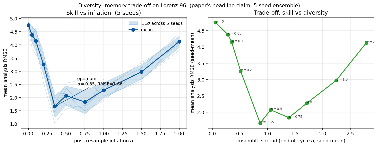
Diversity-memory trade-off on Lorenz-96

The paper’s central finding is that post-resampling inflation sits on a trade-off: without it, the resampled ensemble is all duplicates and the filter collapses; with too much of it, the inflation noise erases the very memory the filter has accumulated from past observations. The result is a U-shaped skill curve with a narrow optimum.

On Lorenz-96, running the same recipe (η = 4 observation-error tempering, max-weight cap 0.3, N = 400 members, observation interval 0.05) and sweeping the post-resampling Gaussian inflation σ from 0 to 2 yields exactly this U-curve. The sweep is repeated across five independent rng seeds so the curve we show is a mean ± 1σ envelope, not a single realisation:

σ inflation	RMSE mean ± σ	resample fraction
0.00	4.75 ± 0.09	0.11 (collapsed)
0.20	3.26 ± 0.38	0.87
0.35	1.66 ± 0.41	0.94
0.50	2.07 ± 0.37	0.99
0.75	1.83 ± 0.44	0.99
1.00	2.28 ± 0.28	0.99
2.00	4.12 ± 0.21	0.99 (noise-dominated)

The envelope is narrow at the endpoints (both failure modes are robust across seeds) and wider at the optimum (the filter sits on the edge of stability there). The right panel is the same sweep re-parameterised as skill vs achieved diversity: the filter must maintain some ensemble spread to work, but excess spread costs skill.

Script: examples/05_l96_diversity_memory.py.

2. Cycle-length sensitivity — the two intrinsic bounds behind T10 / T11 / T12¶

Cycle-length sensitivity on Lorenz-96

What this figure is (and isn’t)

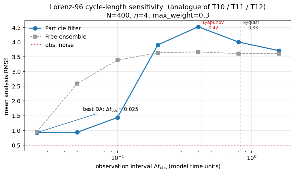
It is not a reproduction of the paper’s AMOC U-curve. It cannot be, for reasons the next paragraphs make precise. It is a direct demonstration that the two intrinsic bounds the paper invokes for AMOC — Lyapunov and Nyquist — are also present on Lorenz-96 with the values the theory predicts. Which of the two dominates the cycle- length curve is a property of the system, not of the filter.

The paper’s observation-interval U-curve on AMOC (T10 = 1 yr marginal, T11 = 5 yr best, T12 = 10 yr degraded by aliasing of the 13.3-year spectral peak) is governed by two intrinsic timescales:

the Lyapunov time \(\tau_L\) — how fast deterministic uncertainty grows between corrections;
the Nyquist bound \(\tau_N = T_\star / 2\) — half the period of the dominant spectral mode.

An observation interval larger than \(\min(\tau_L, \tau_N)\) breaks the filter. On AMOC the coupled-system Lyapunov time is decades (ocean memory dominates) whereas the AMOC spectral peak is at 13.3 years, so \(\tau_N \approx 6.7\) yr is the tighter bound. The paper’s T11 optimum is the consequence: 5-year cycles sit just inside the Nyquist-safe window.

On Lorenz-96 (F = 8) we measure both bounds independently:

\(\tau_L \approx 0.42\) (Bocquet & Carrassi, 2017);
\(\tau_N \approx 0.83\), from the spectral peak at \(T_\star \approx 1.65\) identified in section 4 below.

Both are marked on the figure. The Lyapunov bound bites first: the filter degrades sharply at observation intervals near 0.4, well inside the Nyquist-safe window. This is the opposite ordering from AMOC, and it is exactly what the paper’s analysis predicts for a system whose chaos horizon is short relative to its oscillation period.

Stated plainly: the paper’s T11 optimum does not appear on L96, and it shouldn’t. The mechanism the paper describes — two bounds, the tighter one wins — is what appears on L96. The figure supports the paper’s argument by verifying a quantitative prediction (L96 should not exhibit the AMOC U-curve, because \(\tau_L < \tau_N\) on L96).

Script: examples/04_l96_cycle_sensitivity.py.

3. Diverse initial conditions — analogue of T13¶

Diverse-IC ensemble on Lorenz-96

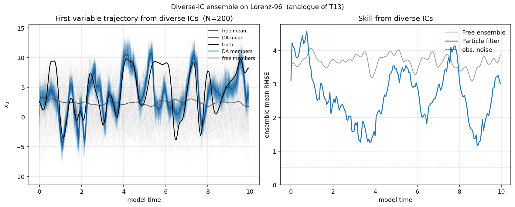
The paper’s T13 ensemble starts each member from a different 50-year slice of a 5000-year control run, spanning AMOC strengths from 17 to 26 Sv. The question it answers is whether the particle filter needs members to share initial-state memory, or whether it can recruit a widely-dispersed ensemble toward the truth using observations alone. T13 shows the latter: with no shared IC, DA achieves strong positive correlation with the truth that the free ensemble cannot.

On Lorenz-96 we spin up each of 200 members from an independent random initial condition, so the initial ensemble is scattered across the attractor. Left: the first state variable over time. The DA ensemble mean (blue) tracks the chaotic truth (black); the free ensemble mean (grey) is pinned near climatology because averaging uncorrelated attractor trajectories returns the attractor mean. Right: RMSE over time. DA pulls the scattered ensemble onto the truth trajectory within a few Lyapunov times.

Script: examples/06_l96_diverse_ics.py.

4. Welch spectrum and the Nyquist argument¶

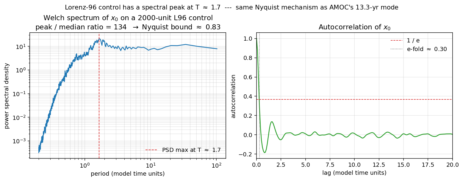
Welch spectrum and autocorrelation of Lorenz-96

Section 4 of the paper computes a Welch spectrum of a 1500-year control integration of the CM2Mc-BLING AMOC time series, identifies a dominant oscillation at ~13.3 years, and uses half of that period (~6.7 years) as a Nyquist bound on the maximum useful assimilation cycle.

The same analysis on a 2000-unit Lorenz-96 control (F = 8, sampling every 0.1 model time units) finds a genuine spectral peak at T ≈ 1.65 with peak / median power ratio ≈ 134. By construction the Nyquist bound is T / 2 ≈ 0.83 — the same grey dotted line overlaid on the cycle-sensitivity figure above.

The autocorrelation panel is an independent sanity check. The e-fold time is 0.30 — tight, consistent with the Lyapunov-limited predictability horizon. The ACF then oscillates with period ≈ 1.65, matching the spectrum.

So Lorenz-96 carries the same Nyquist mechanism the paper invokes for AMOC; the difference is which of the two intrinsic bounds is binding in which regime.

Script: examples/07_l96_nyquist.py.

What this tutorial is for¶

For paper reviewers — a laptop-runnable demonstration that the algorithmic contributions of the paper are implementable outside POEM / CM2Mc-BLING and that they produce the expected filter behaviour on a standard benchmark.
For future users of pypfda — a gallery of canonical experimental setups, each <200 lines, that can be adapted to a different forward model by replacing the integrate() call.
For ourselves — an always-on regression check. If a future refactor of the core ParticleFilter class breaks the diversity-memory U-curve or the cycle-sensitivity shape, it shows up immediately in the rebuilt figures.